#32 ● Cách Sử Dụng Name Range Trong Excel, Đặt Tên Cho Vùng Dữ Liệu

If you are working with Excel spreadsheets, it could mean a lot of time saving and efficiency.

Đang xem: #32 ● cách sử dụng name range trong excel, đặt tên cho vùng dữ liệu

In this tutorial, you’ll learn how to create Named Ranges in Excel and how to use it to save time.

Benefits of Creating Named Ranges in ExcelHow to Create Named Ranges in ExcelToo Many Named Ranges in Excel? Don’t WorryCreating Dynamic Named Ranges in Excel

Named Ranges in Excel – An Introduction

If someone has to call me or refer to me, they will use my name (instead of saying a male is staying in so and so place with so and so height and weight).

Right?

Similarly, in Excel, you can give a name to a cell or a range of cells.

Now, instead of using the cell reference (such as A1 or A1:A10), you can simply use the name that you assigned to it.

For example, suppose you have a data set as shown below:

In this data set, if you have to refer to the range that has the Date, you will have to use A2:A11 in formulas. Similarly, for Sales Rep and Sales, you will have to use B2:B11 and C2:C11.

While it’s alright when you only have a couple of data points, but in case you huge complex data sets, using cell references to refer to data could be time-consuming.

Excel Named Ranges makes it easy to refer to data sets in Excel.

You can create a named range in Excel for each data category, and then use that name instead of the cell references. For example, dates can be named ‘Date’, Sales Rep data can be named ‘SalesRep’ and sales data can be named ‘Sales’.

You can also create a name for a single cell. For example, if you have the sales commission percentage in a cell, you can name that cell as ‘Commission’.

Benefits of Creating Named Ranges in Excel

Here are the benefits of using named ranges in Excel.

Use Names instead of Cell References

When you create Named Ranges in Excel, you can use these names instead of the cell references.

For example, you can use =SUM(SALES) instead of =SUM(C2:C11) for the above data set.

Have a look at ṭhe formulas listed below. Instead of using cell references, I have used the Named Ranges.

Sum of all the sales done by Tom: =SUMIF(SalesRep,”Tom”,Sales)

You would agree that these formulas are easy to create and easy tounderstand (especially when you share it with someone else or revisit it yourself.

No Need to Go Back to the Dataset to Select Cells

Another significant benefit of using Named Ranges in Excel is that you don’t need to go back and select the cell ranges.

You can just type a couple of alphabets of that named range and Excel will show the matching named ranges (as shown below):

Named Ranges Make Formulas Dynamic

By using Named Ranges in Excel, you can make Excel formulas dynamic.

For example, in the case of sales commission, instead of using the value 2.5%, you can use the Named Range.

Now, if your company later decides to increase thecommission to 3%, you can simply update the Named Range, and all the calculation would automatically update to reflect the new commission.

How to Create Named Ranges in Excel

Here are three ways to create Named Ranges in Excel:

Method #1 – Using Define Name

Here are the steps to create Named Ranges in Excel using Define Name:

Select the range for which you want to create a Named Range in Excel.

Go to Formulas –> Define Name.

In the New Name dialogue box, type the Name you wish to assign to the selected data range. You can specify the scope as the entire workbook or a specific worksheet, If you select a particular sheet, the name would not be available on other sheets.

Click OK.

This will create a Named Range SALESREP.

Method #2: Using the Name Box

Select the range for which you want to create a name (do not select headers). Go to the Name Box on the left of Formula bar and Type the name of the with which you want to create the Named Range.

Note that the Name created here will be available for the entire Workbook. If you wish to restrict it to a worksheet, use Method 1.

Method #3: UsingCreate From Selection Option

This is the recommended way when you have data in tabular form, and you want to create named range for each column/row.

For example, in the dataset below, if you want to quickly create three named ranges (Date, Sales_Rep, and Sales), then you can use the method shown below.

Here are the steps to quickly create named ranges from a dataset:

Select the entire data set (including the headers). Go to Formulas –> Create from Selection (Keyboard shortcut – Control + Shift + F3).It will open the ‘Create Names from Selection’ dialogue box.

In the Create Names from Selection dialogue box, check the options where you have the headers. In this case, we select top row only as the header is in the top row. If you have headers in both top row and left column, you can choose both. Similarly, if your data is arranged when the headers are in the left column only, then you only check the Left Column option.

This will create three Named Ranges – Date, Sales_Rep, and Sales.

Note that it automatically picks up names from the headers. If there are any space between words, it inserts an underscore (as you can’t have spaces in named ranges).

Xem thêm: Cách Cắt Video Trên Youtube Bằng Máy Tính Windows 10 (Mới Nhất 2021)

Naming Convention for Named Ranges in Excel

There are certain naming rules you need to know while creating Named Ranges in Excel:

The first character of a Named Range should be a letter and underscore character(_), or a backslash(). If it’s anything else, it will show an error. The remaining characters can be letters, numbers, special characters, period, or underscore. You can not use names that also represent cell references in Excel. For example, you can’t use AB1 as it is also a cell reference. You can’tuse spaces while creating named ranges. For example, you can’t have Sales Rep as a named range. If you want to combine two words and create a Named Range, use an underscore, period or uppercase characters to create it. For example, you can have Sales_Rep, SalesRep, or SalesRep. While creating named ranges, Excel treats uppercase and lowercase the same way. For example, if you create a named range SALES, then you will not be able to create another named range such as ‘sales’ or ‘Sales’. A Named Range can be up to 255 characterslong.

Too Many Named Ranges in Excel? Don’t Worry

Sometimes in large data sets and complex models, you may end up creating a lot of Named Ranges in Excel.

What if you don’t remember the name of the Named Range you created?

Don’t worry – here are some useful tips.

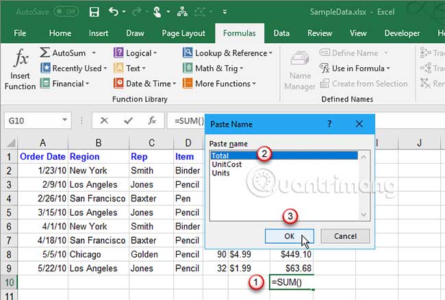
Getting the Names of All the Named Ranges

Here are the steps to get a list of all the named ranges you created:

Go to the Formulas tab. In the Defined Named group, click on Use in Formula.

Click on ‘Paste Names’.

This will give you a list of all the Named Ranges in that workbook. To use a named range (in formulas or a cell), double click onit.

Displaying the Matching Named Ranges

If you have some idea about the Name, type a few initial characters, and Excel will show a drop down of the matching names.

How to Edit Named Ranges in Excel

If you have already created a Named Range, you can edit it using the following steps:

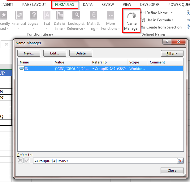
Go to the Formulas tab and click on Name Manager.

The Name Manager dialog box will list all the Named Ranges in that workbook. Double click on the Named Range that you want to edit.

In the Edit Name dialog box, make the changes.

Click OK. Close the Name Manager dialog box.

Useful Named Range Shortcuts (the Power of F3)

Here are some useful keyboard shortcuts that will come handy when you are working with Named Ranges in Excel:

To get a list of all the Named Ranges and pasting it in Formula:F3 To create new name using Name Manager Dialogue Box:Control + F3 To create Named Ranges from Selection: Control + Shift + F3

Creating Dynamic Named Ranges in Excel

So far in this tutorial, we have created static Named Ranges.

This means that these Named Ranges would always refer to the same dataset.

For example, if A1:A10 has been named as ‘Sales’, it would always refer to A1:A10.

If you add more sales data, then you would have to manually go and update the reference in the named range.

In the world of ever-expanding data sets, this may end up taking up a lot of your time. Every time you get new data, you may have to update the Named Ranges in Excel.

To tackle this issue, we can create Dynamic Named Ranges in Excel that would automatically account for additional data and include it in the existing Named Range.

For example,For example, if I add two additional sales data points, a dynamic named range would automatically refer to A1:A12.

This kind of Dynamic Named Range can be created by using Excel INDEX function. Instead of specifying the cell references while creating the Named Range, we specify the formula. The formula automatically updated when the data is added or deleted.

Let’s see how to create Dynamic Named Ranges in Excel.

Suppose we have the sales data in cell A2:A11.

Here are the steps to create Dynamic Named Ranges in Excel:

Go to the Formula tab and click on Define Name.

In the New Name dialogue box type the following: Name:Sales Scope: Workbook Refers to: =$A$2:INDEX($A$2:$A$100,COUNTIF($A$2:$A$100,””&””))

Click OK.

Done!

You now have a dynamic named range with the name ‘Sales’. This would automatically update whenever you adddata to it or remove data from it.

How does Dynamic Named Ranges Work?

To explain how this work, you need to know a bit more about Excel INDEX function.

Most people use INDEX to return a value from a list based on the row and column number.

But the INDEX function also has another side to it.

It can be used to return a cell reference when it is used as a part of a cell reference.

For example, here is the formula that we have used to create a dynamic named range:

=$A$2:INDEX($A$2:$A$100,COUNTIF($A$2:$A$100,””&””)) INDEX($A$2:$A$100,COUNTIF($A$2:$A$100,””&””)–> This part of the formula is expected to return a value (which would be the 10th value from the list, considering there are ten items).

However, when used in front of a reference (=$A$2:INDEX($A$2:$A$100,COUNTIF($A$2:$A$100,””&””))) it returns the reference to the cell instead of the value.

Hence, here it returns =$A$2:$A$11

If we add two additional values to the sales column, it would then return =$A$2:$A$13

When you add new data to the list, Excel COUNTIF function returns the number of non-blank cells in the data. This number is used by the INDEX function to fetch the cell reference of the last item in the list.

Xem thêm: Giải Phương Trình Bậc 2 Logarit, Đk Học Toán: 0946

Note:

This would only work if there are no blank cells in the data. In the example taken above, I have assigned a large number of cells (A2:A100) for the Named Range formula. You can adjust this based on your data set.

You can also use OFFSET function to create a Dynamic Named Ranges in Excel, however, since OFFSET function is volatile, it may lead a slow Excel workbook. INDEX, on the other hand, is semi-volatile, which makes it a better choice to create Dynamic Named Ranges in Excel.