How To Use The Excel Ln Function, Ms Excel: How To Use The Ln Function (Ws)

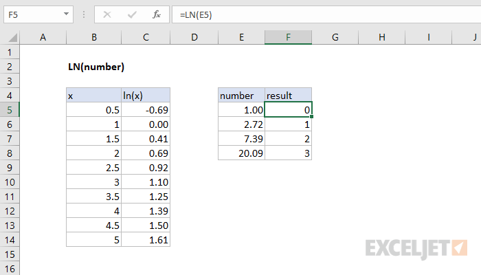
LN function in Excel is designed to calculate the natural logarithm of a number and returns the corresponding numeric value. The natural logarithm is the logarithm with base e (Euler number is approximately 2.718).

Đang xem: How to use the excel ln function

LOG function in Excel is used to calculate the logarithm of a number, and the base of the logarithm can be specified explicitly as the second argument to this function.

LOG10 function in Excel is designed to calculate the logarithm of a number with a base of 10 (decimal logarithm).



Examples of using LN, LOG and LOG10 functions in Excel

Example 1. Archaeologists have found the remains of an ancient animal. To determine their age, it was decided to use the method of radiocarbon analysis. As a result of measurements, it turned out that the content of the radioactive isotope C14 was 17% of the amount that is usually found in living organisms. Calculate the age of the remains, if the half-life of the carbon isotope 14 is 5760 years.

View source table:

To solve, use the following formula:

This formula was derived from the formula x = t * (lgB-lgq) / lgp, where:

q is the amount of carbon isotope at the initial moment (at the time of death of the animal), expressed by a unit (or 100%);B is the amount of isotope at the time of the analysis of the remains;t is the half-life of the isotope;p is a numeric value indicating how many times the amount of a substance (carbon isotope) changes over a period of time t.

As a result of the calculations we get:

Found remains of almost 15 thousand years.



Deposit calculator with compound interest in Excel

Example 2. A bank customer made a deposit in the amount of 50,000 with an interest rate of 14.5% (compound interest). Determine how much time it will take to double the amount invested?

Interesting fact! For a quick solution of this problem, you can use the empirical method of approximate estimation of terms (in years) for doubling investments invested under compound interest. The so-called rule 72 (or 70 or rule 69). To do this, use a simple formula – the number 72 is divided by the interest rate: 72 / 14.5 = 4.9655 years. The main drawback of the rule of the “magic” number 72 is in the error. The higher the interest rate, the higher the error in rule 72. For example, with an interest rate of 100% per annum, the error in years reaches 0.72 (and in percentage this is as much as 28%!).

To accurately calculate the doubling of investment terms, we will use the LOG function. For one thing and check the error of the rule 72 at an interest rate of 14.5% per annum.

View source table:

To calculate the future value of an investment at a known interest rate, you can use the following formula: S=A(100%+n%)t , where:

S is the expected amount upon expiration;A – deposit size;n is the interest rate;t – the period of storage of deposit funds in the bank.

For this example, this formula can be written as 100000 = 50000*(100% + 14.5%)t or 2 = (100% + 14.5%)t . Then, to find t, you can rewrite the equation as t = log(114.5%) 2 or t = log1,1452.

To find the value of t, we write the following formula for compound interest on a deposit in Excel:

=LOG(B4/B2,1+B3)

Argument Description:

B4 / B2 – the ratio of the expected and initial amounts, which is an indicator of the logarithm;1 + B3 – percentage increase (base of logarithm).

As a result of the calculations we get:

The deposit will double in a little over 5 years. To accurately determine the years and months, we use the formula:

TRUNC function discards in a fractional number everything that is after the comma, like the whole INT function. The difference between the functions of the TRUNC and the INT is only in the calculations with negative fractional numbers. In addition, TRUNC has a second argument where you can specify the number of decimal places to be left. The poet in this case, you can use either of these two functions to the user”s choice.

Xem thêm: Soạn Bài Lập Dàn Ý 1 Bài Văn Nghị Luận Xã Hội: Các Dạng Bài Phổ Biến

It turned out 5 years and 1 month and 12 days. Now we compare the exact results with rule 72 and determine the magnitude of the error. For this example, the formula is as follows:

=72/(B3*100)

We have to multiply the value of cell B3 by 100, since its current value is 0.145, which is displayed in percentage format. As a result:

Then copy the formula from cell B6 to cell B8, and in cell B9:

Calculate the timing of error:

=B5-B7

Then in cell B10, copy the formula from cell B6 again. As a result, we get the difference:

Finally, we calculate the difference in percentages in order to check how the size of the deviation changes and how significantly the growth of the interest rate influences the level of divergence of rule 72 and the fact:

Now, for clarity, the proportional dependence of the increase in error and the growth of the interest rate will raise the interest rate to 100% per annum:

At first glance, the margin of error is insignificant compared to 14.5% per annum – only about 2 months and 100% per annum – within 3 months. But the proportion of error in the payback period of more than ¼, or rather 28%.

Let”s make a simple graph for visual analysis of how the dependence of the change in the interest rate and the error percentage of rule 72 on the fact correlates:

The higher the interest rate, the worse the rule 72 works. As a result, the following conclusion can be made: up to 32.2% per annum, you can safely use rule 72. Then the error is less than 10 percent. It will be fine if you do not require accurate, but complex calculations on the payback period of investments by 2 times.

Investment calculator of compound interest with capitalization in Excel

Example 3. A bank client was offered to make a deposit with a continuous increase in the total amount (capitalization with compound interest). The interest rate is 13% per annum. Determine how long it takes to triple the initial amount 250,000. How much is necessary to increase the interest rate to reduce the waiting time by half?

Note: since in this example we are reducing the amount of investments, here rule 72 does not work.

View source data table:

Continuous growth can be described by the formula ln (N) = p * t, where:

N is the ratio of the final amount of the deposit to the initial one;p – interest rate;t is the number of years since the deposit was made.

Then t=ln(N)/p. Based on this equality, we write the formula in Excel:

=LN(B3/B2)/B4

Argument Description:

B3 / B2 – the ratio of the final and initial amount of the deposit;B4 – interest rate.

It will take almost 8.5 years to triple the initial deposit amount. To calculate the rate, which will reduce the waiting time by half, we use the formula:

=LN(B3/B2)/(0.5*B5)

The result:

That is, it is necessary to double the initial interest rate.

Features of using LN, LOG and LOG10 functions in Excel

LN function has the following syntax:

=LN(number)

number is the only argument that is required, which takes real numbers from a range of positive values.

Notes:

LN function is the inverse of the EXP function. The latter returns the value obtained by raising the number e to the specified power. The LN function indicates the degree to which the number e (base) must be raised to obtain the logarithm exponent (argument number).If the argument number is a number from a range of negative values or zero, the result of the LN function is the error code #NUM!.

Syntax of the LOG function is as follows:

=LOG(number,)

Argument Description:

number is a required argument characterizing the numerical value of the logarithm index, that is, the number obtained as a result of raising the base of the logarithm to a certain degree, which will be calculated by the LOG function; is an optional argument describing the numeric value of the base of the logarithm. If the argument is not explicitly specified, the logarithm is considered decimal (that is, the base is 10).

Notes:

Although the result of calculating the LOG function may be a negative number (for example, the function =LOG(2,0.25) returns a value of -0.5), the arguments of this function must be taken from a range of positive values. If at least one of the arguments is a negative number, LOG returns the #NUM! Error code.If the value 1 was passed as an argument to , the LOG function returns the error code #DEL/0!, since the result of raising 1 to any power will always be the same and equal to 1.

LOG10 function has the following syntax entry:

=LOG10(number)

number is the only and required argument, the meaning of which is identical to the argument of the same name of the functions LN and LOG.

Xem thêm: Tổng Hợp 13 Bài Văn Mẫu Lớp 5 Tả Đồ Vật Lớp 5 Hay Nhất, Tả Đồ Vật Lớp 5 Ngắn Gọn Hay Nhất

hướng dẫn examples LN and LOG for calculating natural logarithm in Excel

Note: If a negative number or 0 was passed as an argument, LOG10 returns the error code #NUM!.