How To Create An Excel Dashboard In 7 Steps, Excel Dashboards

A dashboard is a visual representation of key metrics that allow you to quickly view and analyze your data in one place. Dashboards not only provide consolidated data views, but a self-service business intelligence opportunity, where users are able to filter the data to display just what’s important to them. In the past, Excel reporting often required you to generate multiple reports for different people or departments depending on their needs.

Đang xem: How to create an excel dashboard in 7 steps

Overview

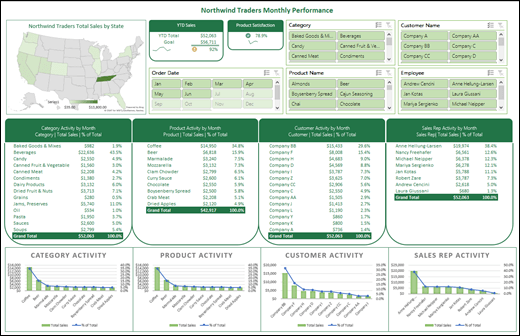
In this topic, we’ll discuss how to use multiple PivotTables, PivotCharts and PivotTable tools to create a dynamic dashboard. Then we”ll give users the ability to quickly filter the data the way they want with Slicers and a Timeline, which allow your PivotTables and charts to automatically expand and contract to display only the information that users want to see. In addition, you can quickly refresh your dashboard when you add or update data. This makes it very handy because you only need to create the dashboard report once.

For this example, we”re going to create four PivotTables and charts from a single data source.

Once your dashboard is created, we’ll show you how to share it with people by creating a lingocard.vn Group. We also have an interactive Excel workbook that you can hướng dẫn and follow these steps on your own.

hướng dẫn the Excel Dashboard tutorial workbook.

Create a dashboard Share your dashboard


Get your data

You can copy and paste data directly into Excel, or you can set up a query from a data source. For this topic, we used the Sales Analysis query from the Northwind Traders template for lingocard.vn Access. If you want to use it, you can open Access and go to File > New > Search for “Northwind” and create the template database. Once you’ve done that you’ll be able to access any of the queries included in the template. We’ve already put this data into the Excel workbook for you, so there’s no need to worry if you don’t have Access.

Create PivotTables

Once you”ve created your master PivotTable, select it, then copy and paste it as many times as necessary to empty areas in the worksheet. For our example, these PivotTables can change rows, but not columns so we placed them on the same row with a blank column in between each one. However, you might find that you need to place your PivotTables beneath each other if they can expand columns.

Important: PivotTables can”t overlap one another, so make sure that your design will allow enough space between them to allow for them to expand and contract as values are filtered, added or removed.

At this point you might want to give your PivotTables meaningful names, so you know what they do. Otherwise, Excel will name them PivotTable1, PivotTable2 and so on. You can select each one, then go to PivotTable Tools > Analyze > enter a new name in the PivotTable Name box. This will be important when it comes time to connect your PivotTables to Slicers and Timeline controls.

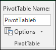
Analyze > PivotTable Name box” />

Create PivotCharts

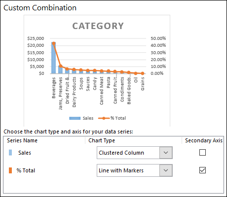
Click anywhere in the first PivotTable and go to PivotTable Tools > Analyze > PivotChart > select a chart type. We chose a Combo chart with Sales as a Clustered Column chart, and % Total as a Line chart plotted on the Secondary axis.

Repeat for each of the remaining PivotTables.

Now is a good time to rename your PivotCharts too. Go to PivotChart Tools > Analyze > enter a new name in the Chart Name box.

Add Slicers and a Timeline

Slicers and Timelines allow you to quickly filter your PivotTables and PivotCharts, so you can see just the information that”s meaningful to you.

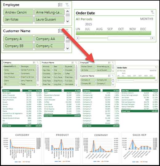
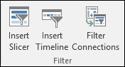
Select any PivotTable and go to PivotTable Tools > Analyze > Filter > Insert Slicer, then check each item you want to use for a slicer. For this dashboard, we selected Category, Product Name, Employee and Customer Name. When you click OK, the slicers will be added to the middle of the screen, stacked on top of each other, so you’ll need to arrange and resize them as necessary.

Analyze > Filter” />

Slicer Options – If you click on any slicer, you can go to Slicer Tools > Options and select various options, like Style and how many columns are displayed. You can align multiple slicers by selecting them with Ctrl+Left-click, then use the Align tools on the Slicer Tools tab.

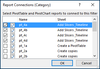
Slicer Connections – Slicers will only be connected to the PivotTable you used to create them, so you need to select each Slicer then go to Slicer Tools > Options > Report Connections and check which PivotTables you want connected to each. Slicers and Timelines can control PivotTables on any worksheet, even if the worksheet is hidden.

Options” />

Add a Timeline – Select any PivotTable and go to PivotTable Tools > Analyze > Filter > Insert Timeline, then check each item you want to use. For this dashboard, we selected Order Date.

Xem thêm: Những Bài Văn Nghị Luận Xã Hội Hay Lớp 12, Tuyển Tập 36 Đề Văn Nghị Luận Xã Hội Hay

Timeline Options – Click on the Timeline, and go to Timeline Tools > Options and select options like Style, Header and Caption. Select the Report Connections option to link the timeline to the PivotTables of your choice.

Learn more about Slicers and Timeline controls.

Next steps

Your dashboard is now functionally complete, but you probably still need to arrange it the way you want and make final adjustments. For instance, you might want to add a report title, or a background. For our dashboard, we added shapes around the PivotTables and turned off Headings and Gridlines from the View tab.

Make sure to test each of your slicers and timelines to make sure that your PivotTables and PivotCharts behave appropriately. You may find situations where certain selections cause issues if one PivotTable wants to adjust and overlap another, which it can’t do and will display an error message. These issues should be corrected before you distribute your dashboard.

Once you’re done setting up your dashboard, you can click the “Share a Dashboard” tab at the top of this topic to learn how to distribute it.

Congratulations on creating your dashboard! In this step we”ll show you how to set up a lingocard.vn Group to share your dashboard. What we”re going to do is pin your dashboard to the top of your group”s document library in SharePoint, so your users can easily access it at any time.

Store your dashboard in the group

If you haven”t already saved your dashboard workbook in the group you”ll want to move it there. If it”s already in the group”s files library then you can skip this step.

Go to your group in either Outlook 2016 or Outlook on the web.

Click Files in the ribbon to access the group”s document library.

Click the Upload button on the ribbon and upload your dashboard workbook to the document library.

Add it to your group”s SharePoint Online team site

If you accessed the document library from Outlook 2016, click Home on the navigation pane on the left. If you accessed the document library from Outlook on the web, click More > Site from the right end of the ribbon.

Click Documents from the navigation pane at the left.

Find your dashboard workbook and click the selection circle just to the left of its name.

When you have the dashboard workbook selected, choose Pin to top on the ribbon.

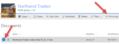
Now whenever your users come to the Documents page of your SharePoint Online team site your dashboard worksheet will be right there at the top. They can click on it and easily access the current version of the dashboard.

Xem thêm: Mbti, Trắc Nghiệm Tính Cách Mbti, Chọn Nghề Nghiệp Miễn Phí Chuẩn 2021

Tip: Your users can also access your group document library, including your dashboard workbook, via the Outlook Groups mobile app.